Frank’s Goldfish Projects - Work with AMES Data

library(tidyverse)
library(tidymodels)
theme_set(theme_minimal())

ames <- mutate(ames, Sale_Price = log10(Sale_Price))

Study Features

My first intuition is create a factor analysis so I can try understand which dimensions are related which are not.

Explore data using pca for analysing top performing featuresfviz_pca_ind

ames.numb = ames |> 
  select(where(is.numeric)) |> 
  select(-starts_with("Year_"), -Longitude, - Latitude, -Sale_Price)

# ames.numb |> glimpse()

ames.fct = ames.numb |> 
  prcomp(scale=T) # the function

# # fviz_eig from factoextra package
library(factoextra)

Welcome! Want to learn more? See two factoextra-related books at https://goo.gl/ve3WBa

ames.fct |> fviz_eig() #Extract and visualize the eigenvalues/variances of dimensions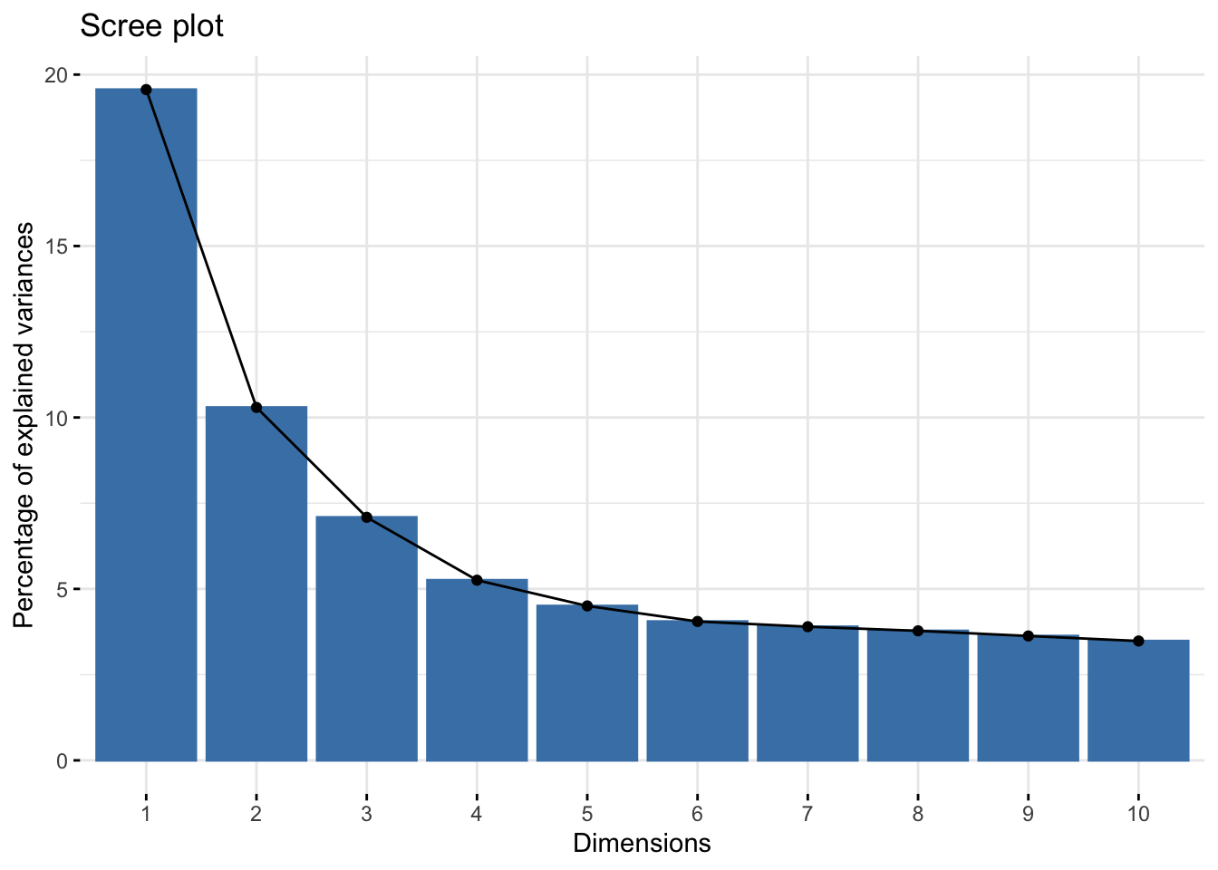

From this plot the elbow seems to be two or three. This visualization seems to be better at explaining factors (I will continue my fascination with PCA later).

fviz_pca_var(
  ames.fct
  ,col.var = "contrib"
  ,gradient.cols = c("#00AFBB", "#E7B800", "#FC4E07")
  ,repel = TRUE     # Avoid text overlapping
  )

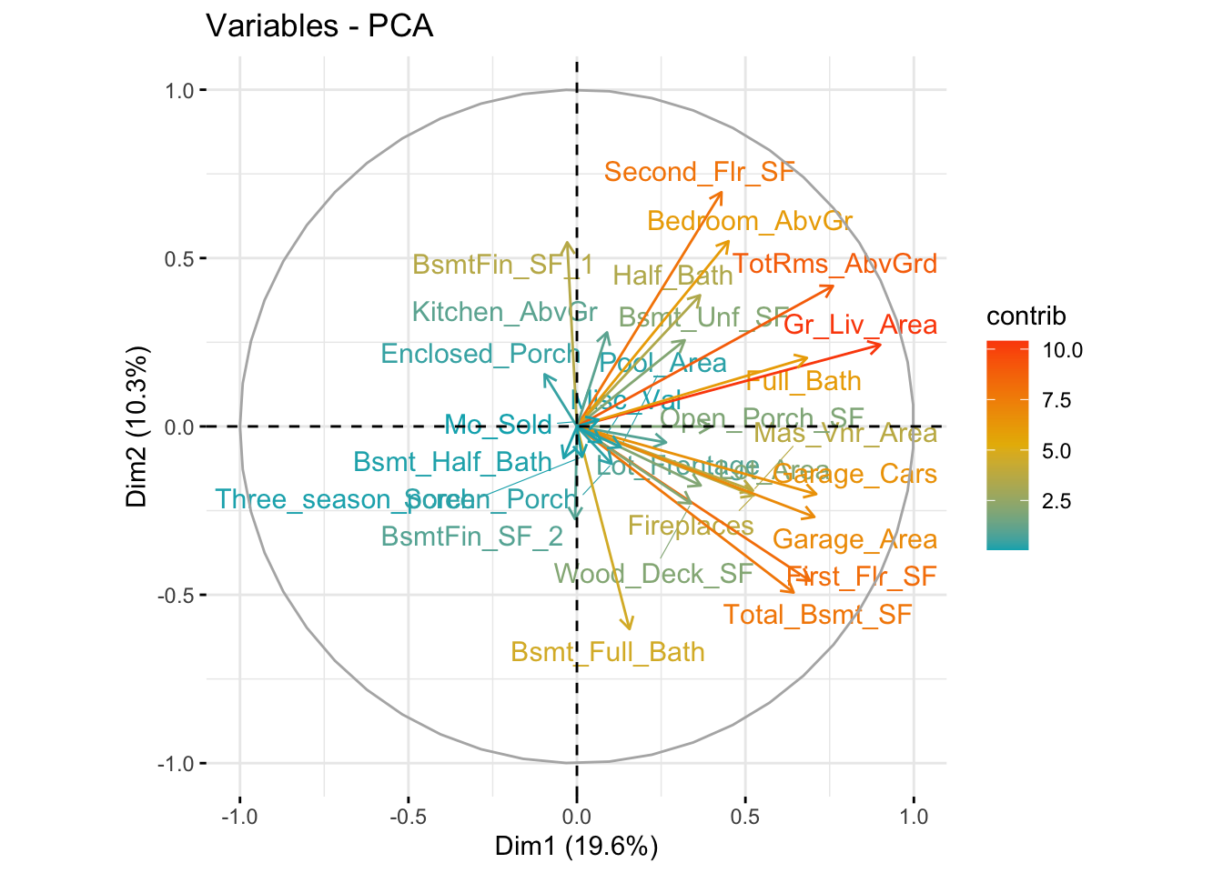
Actually you can use PCA with tidy-model (because you can also train and predict)

ames_tts = ames |> initial_split(prop = 0.8, strata = Sale_Price)
ames_train = ames_tts |> training()
ames_test = ames_tts |> testing()

pca_trans = ames_train |> 
  select(where(is.numeric)) |> 
  recipe(~.) |> 
  step_normalize(all_numeric()) |> 
  step_pca(all_numeric(), num_comp = 2)# still

Getting data out, according to receipt example, instead of train or predict you do so by prep and bake.

This results in scoring of the two latent feature for each individual row.

#
pca_estimate = pca_trans |> prep()
pca_data <- bake(pca_estimate,ames_train)
pca_data

# A tibble: 2,342 × 2
     PC1    PC2
   <dbl>  <dbl>
 1  2.52  0.852
 2  2.11  2.60 
 3  3.33  0.465
 4  2.69 -0.510
 5  2.42 -1.40 
 6  2.72 -1.75 
 7  1.10  1.38 
 8  3.28  0.290
 9  2.02  0.177
10  3.57 -0.204
# ℹ 2,332 more rows

Extract coeficient feature for against all score?

## visualise coeficiency results
require(tidytext)

Loading required package: tidytext

tidy(pca_estimate,number=2,type="coef") |> 
  filter(component %in% c("PC1","PC2")) |> 
  ggplot(aes(x = value, y=terms, fill=component)) +
  geom_col() + 
  scale_fill_brewer(palette = "Set1") + 
  ggtitle("Extracting Feature from Tidyverse Principle Component")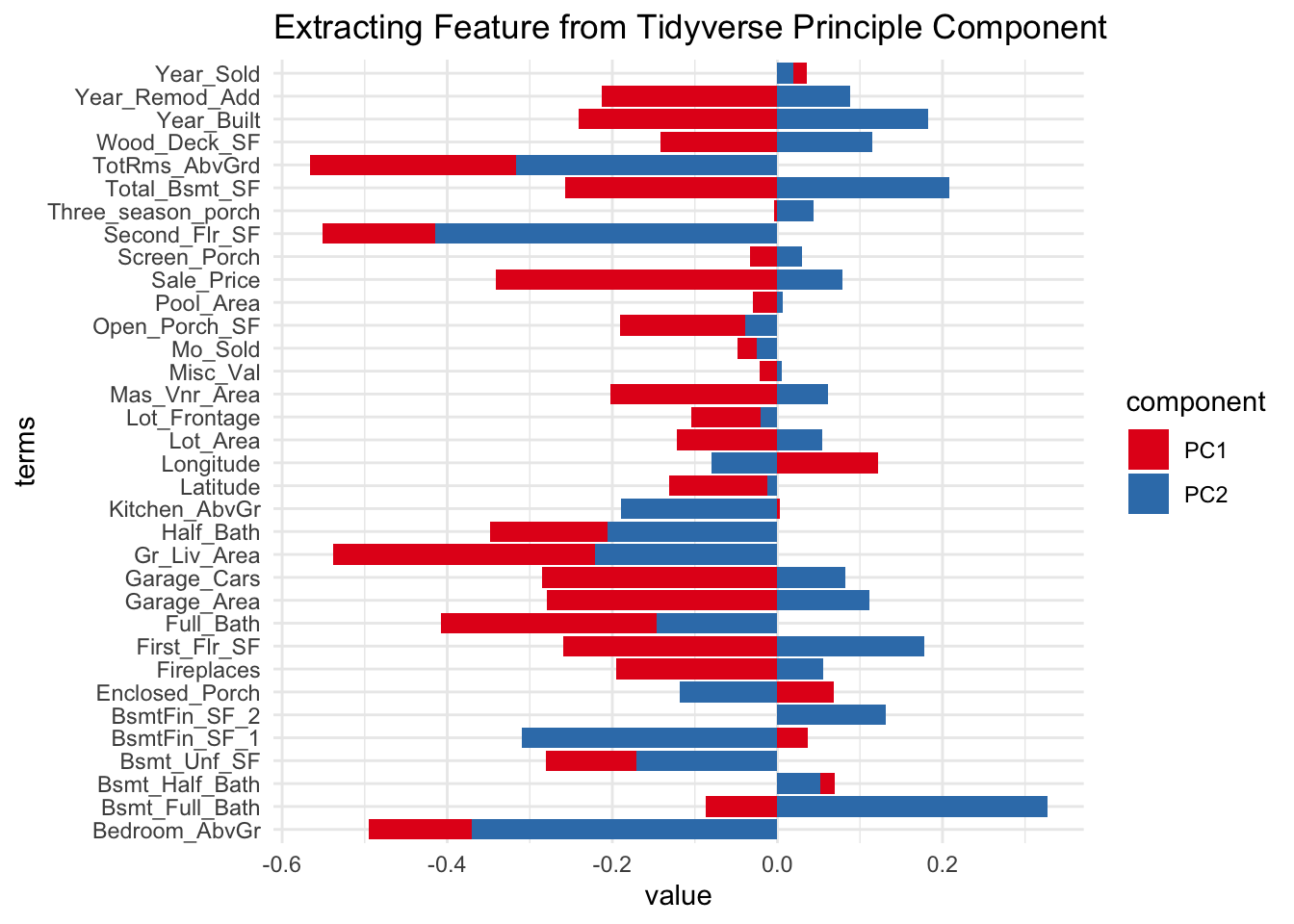

By calculating corelation matrix is indeed, you replicate the same value from the latent feature.

X <- ames_train |> select(where(is.numeric), -Sale_Price)

cor(X, pca_data ) |> 
  data.frame() |> 
  rownames_to_column() |> 
  pivot_longer(c(PC1, PC2)) |> 
  ggplot(aes(y=rowname, x=value, fill=name)) + 
  geom_col() + 
  ggtitle("Calcuate Corelation Matrix from Scratch")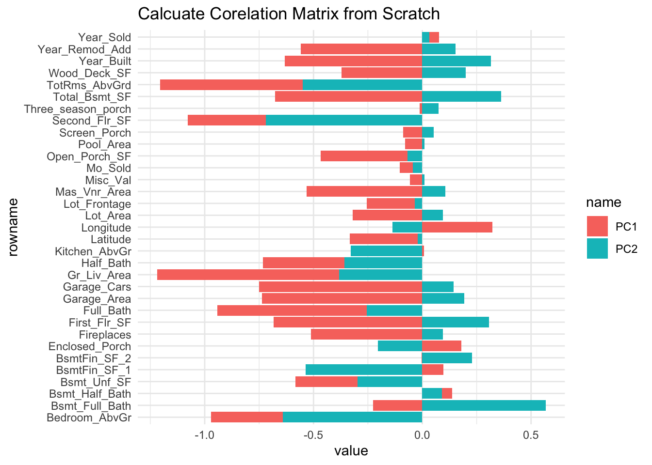

tidy(pca_estimate,number=2,type="variance") |> 
  ggplot(aes(y = value, x = component,fill=terms)) + 
  geom_col() + 
  facet_wrap(~terms,scales = "free")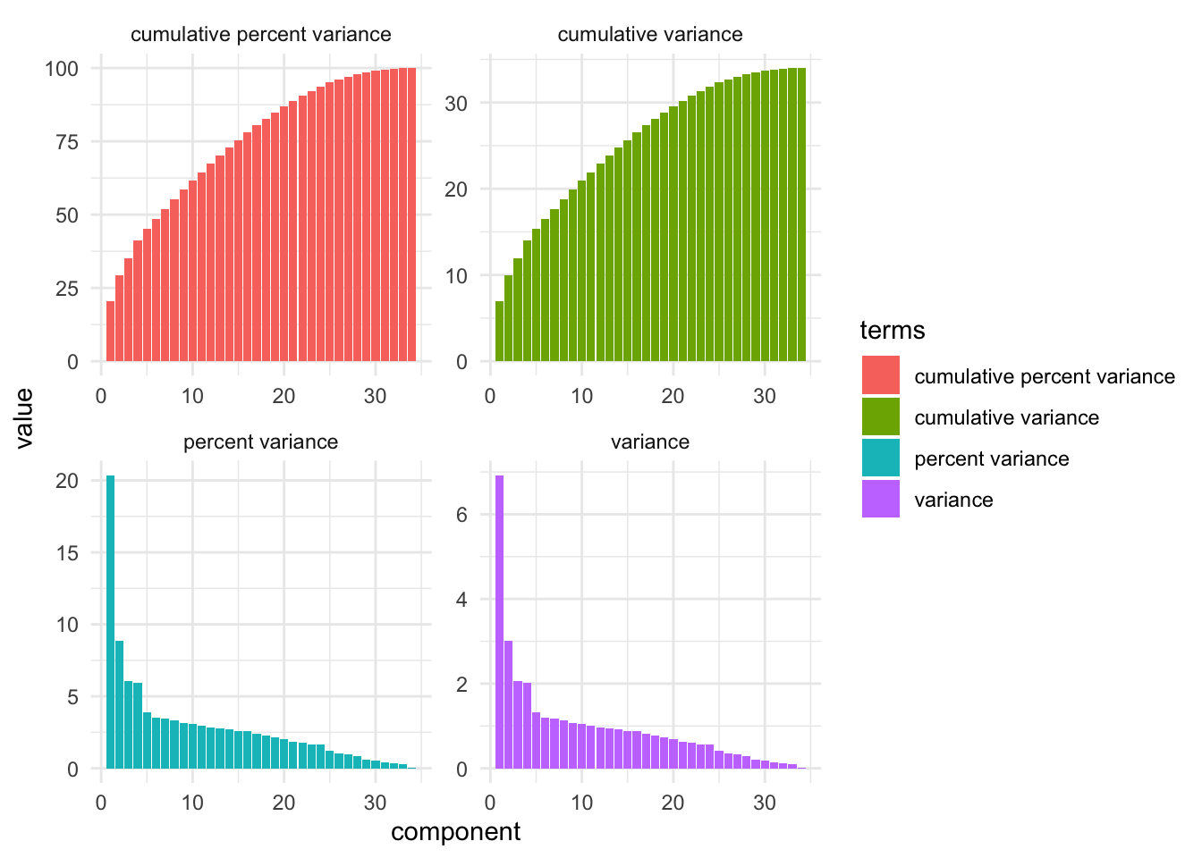

Experimenting closest feature.

However I am interested in see which feature should below in which under laying factor?

So I created this visualisaion:

magic function for compare features

compare_factor = function(tidybaked, pca1, pca2) {
  
  pca1Quo = quo(get(pca1))
  pca2Quo = quo(get(pca2))
  
  tidybaked |> 
    filter(component %in% c(pca1,pca2)) |> 
    pivot_wider(
       names_from=component
      ,values_from=value
    ) |> 
    mutate(diff = !!pca2Quo - !!pca1Quo) |> 
    arrange(diff) |> 
    rowwise() |> 
    mutate(
      mxv=max(!!pca2Quo, !!pca1Quo), miv=min(!!pca2Quo, !!pca1Quo)
    ) |>
    mutate(
       terms = fct_inorder(terms)
      ,is_pc2=diff >= 0
      ,abs_diff=abs(diff)) |> 
    ggplot(aes(y= terms,alpha=abs_diff)) + 
    geom_linerange(
      aes(xmin=miv,xmax=mxv,color=is_pc2)
      ,linewidth=2
      ) + 
    geom_point(aes(x=!!pca1Quo),color="lightcoral") + 
    geom_point(aes(x=!!pca2Quo),color="cyan3") +
    scale_alpha_continuous(trans="sqrt") +
    theme(legend.position="none")
}

This compares principle component 1 against 2

tidy(pca_estimate,number=2,type="coef") |> 
  compare_factor("PC1", "PC2") +
  ggtitle(
    "Feature Alocation of two principle component"
    ,"Compare coeficency of PCA1 against PCA2")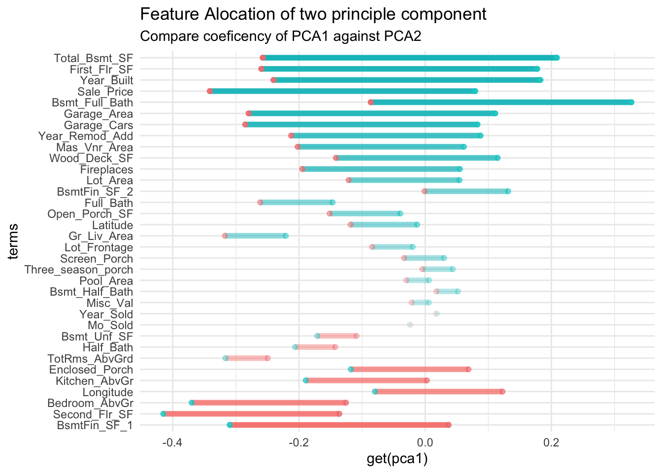

This compares principle component from 2 against 3

tidy(pca_estimate,number=2,type="coef") |> 
  compare_factor("PC2", "PC3") +
  ggtitle(
    "Feature Aloocation of two principle component"
    ,"Compare PCA2 against PCA3")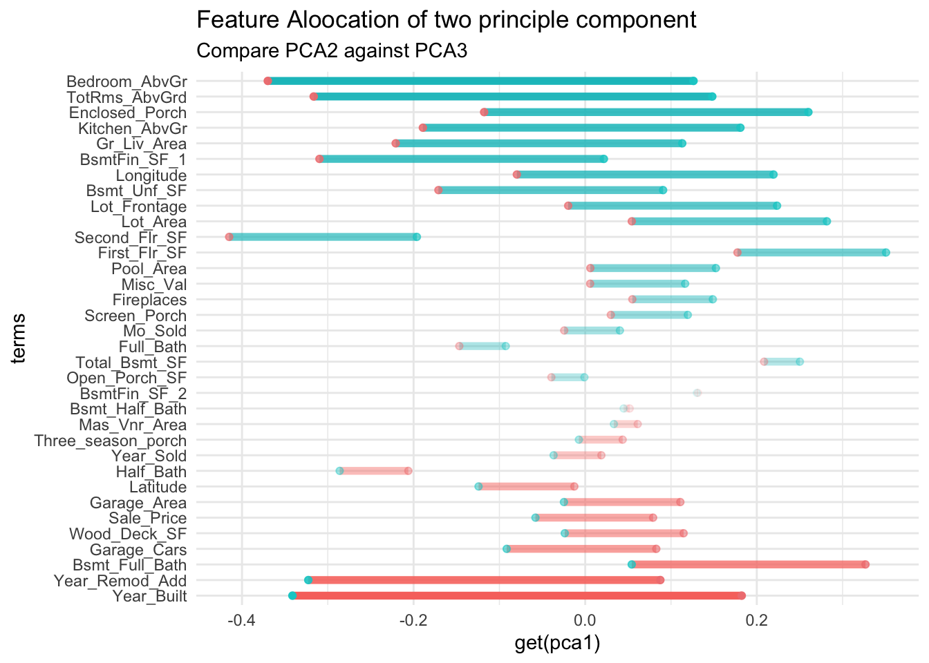

However I don’t understand this visualisation enough to understand if what this PCA says about data (if they are latend or not). So I am creating below experiment to understand PCA.

Experiment of a rotated 2D surface in a 3D surfaces

First is by creating on latent variable we understand.

If project a 2D sheet in a 3D space the surface point on that 2D sheet has underlaying latent space of the 2 dimension.

First we need to sample a surface point and rotate this surface

x <- rnorm(1000)
y <- rnorm(1000)

d = data.frame(
   x = x
  ,y = y 
) |> 
  arrange(x) |> 
  mutate(z = x + y)
plotly::plot_ly(d
  ,x=~x
  ,y=~y
  ,z=~z
  ,marker=list(
    color="blue"
    ,size=2))

No trace type specified:
  Based on info supplied, a 'scatter3d' trace seems appropriate.
  Read more about this trace type -> https://plotly.com/r/reference/#scatter3d

No scatter3d mode specifed:
  Setting the mode to markers
  Read more about this attribute -> https://plotly.com/r/reference/#scatter-mode

require(factoextra)
normal_fct = d |> 
  prcomp()

normal_fct |> 
  get_eig()

        eigenvalue variance.percent cumulative.variance.percent
Dim.1 2.912219e+00     7.337731e+01                    73.37731
Dim.2 1.056609e+00     2.662269e+01                   100.00000
Dim.3 8.190886e-31     2.063805e-29                   100.00000

## screen plot is ploting wahts
normal_fct |> 
  fviz_eig()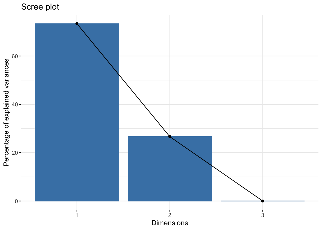

In this case, the true under-laying variance, it depends on how that surface you generated rotate.

normal_fct |> 
  fviz_pca_var(repel=T)

fct_d = d |> 
  recipe() |> 
  step_normalize() |> 
  step_pca()

fct_d |> prep() |> tidy()

# A tibble: 2 × 6
  number operation type      trained skip  id             
   <int> <chr>     <chr>     <lgl>   <lgl> <chr>          
1      1 step      normalize TRUE    FALSE normalize_LECN5
2      2 step      pca       TRUE    FALSE pca_27riA

Actual Model

## classic geo-special machine-learning traning
ames_rec = ames_train |> 
  recipe(Sale_Price ~ 
           Neighborhood 
         + Gr_Liv_Area 
         + Year_Built 
         + Bldg_Type
         + Latitude 
         + Longitude, data=ames_train) |> 
  step_log(Gr_Liv_Area, base=10) |> 
  step_other(Neighborhood, threshold=0.01) |> 
  step_dummy(all_nominal_predictors()) |> 
  step_interact( ~ Gr_Liv_Area:starts_with("Bldg_Type_")) |> 
  step_ns(Latitude,Longitude,deg_free=20)
  
lm_model=linear_reg() |> set_engine("lm")
tree_model=rand_forest() |> 
  set_engine("ranger") |> 
  set_mode("regression")


## base line for use single model
lm_wflow =
  workflow() |> 
  add_model(lm_model) |> 
  add_recipe(ames_rec)

## use multiple model requires receipy and model match up
wflowset = workflow_set(
  list(ames_rec), 
  models=list(lm_model, tree_model))

wflowset |> 
  workflow_map() |> 
  mutate(fitted = map(info, ~ fit(.x$workflow[[1]],ames_train) ))

✖ The workflow requires packages that are not installed: 'ranger'. Skipping this workflow.

Error in `mutate()`:
ℹ In argument: `fitted = map(info, ~fit(.x$workflow[[1]], ames_train))`.
Caused by error in `map()`:
ℹ In index: 2.
Caused by error in `fit_xy()`:
! Please install the ranger package to use this engine.

You won’t be able to fit model because you have not learned re-sample yet.